Overview
This is a hands-on introduction to VLBI data reduction using CASA. The tutorial is based on previous tutorials from the DARA tutorial and the ERIS 2024 tutorials. We have adapted them for the EVN observations with project code RSM07, that was observed during the e-EVN run on 16 September 2025 (during the school).
About the EVN data to calibrate
We are going to work with the project RSM07. As aforementioned, this is a short EVN observation taken during the e-EVN run on 16 September 2025 at L band (1.67 GHz).
For context, this is the summary of this observation:
Observation: RSM07
Mode:Continuum phase-referencing dataset
Duration: 3 hours
Method: Telescopes nodding between calibrator (C) and target (T) in C-T-C-T pattern
| Source Type | Source Name |
|---|---|
| Calibrator (C) | J1848+3219 |
| Target (T) |
3C395 |
| Fringe-finder (FF) |
3C345 |
The data and related information can be accessed from the EVN Data Archive, selecting the project "RSM07". Or directly, going to the experiment-related page.
In a regular EVN observation, the principal investigator (PI) receives an email with the basic information about the observation, together with the credentials to access the data (the same sent to all participants during the school). This information can always be retrieved by going, in the Archive pages to Standard Plots -> Letter to the P.I.
In this page ('Standard Plots'), you can see the following information:
- The PI's surname is Marcote.
- The observations were taken at a central wavelength of 18 cm (1.67 GHz).
- The stations (antennas) that were scheduled were: Jb (Jodrell Bank Mark II, UK), Wb (Westerbork, The Netherlands), Ef (Effelsberg, Germany), Mc (Medicina, Italy), O8 (Onsala, Sweden), T6 (Tianma, China), Tr (Torun, Poland), Hh (Harteebesthoek, South Africa), Ir (Irbene, Latvia), Cm (Cambridge, eMERLIN, UK), Da (Darnhall, eMERLIN, UK), Kn (Knocking, eMERLIN, UK), Pi (Pickmere, eMERLIN, UK), De (Deffort, eMERLIN, UK).
- The shown plots can be useful to understand the data even before downloading it (they contain the data as outputed from the correlator, before any calibration).
From the PI letter, we can see that the correlated data will contain: 13 Antennas, 4 subbands, each with 4 pols and 64 spectral channels; 2-sec integrations. And the following information are included for the different antennas:
- O8: Stowed due to strong winds.
- Tr: Could not observe.
- Cm: No fringes during the observation.
- Da: Could not observe.
- Kn: No fringes during the observation.
- Pi: No fringes during the observation.
- De: No fringes between 13:45-15:03 UT.
This means that we may expect to see data from these antennas but we should directly flag them as they will not be providing useful data. Additionally, the PI letter mentions that Cm, Kn, Pi, De only observed subbands 2-3, due to their local bandwidth limitations.
The 'Pipeline calibration' section takes you to the inputs and outputs from the EVN Pypeline. Here you can see an extensive collection of plots from the different calibration steps, some preliminary images from the sources, and the calibrated (uv) data (visibilities), in UVFITS format. However, note that the current pipeline is far from providing reliable results and thus these data should not be used for science. But they are often helpful to see what may the expected outcome of the observations.
Data Download
From the same RSM07 page in the EVN Archive, and going to the 'Fitsfiles' section, you will see the command that allows you to download the data (which is divided in two FITS-IDI files).
If you are requested for a password, then the credentials for accessing the data are:
username: rsm07
password: m7PQOTdy2Mgl
Another related files are required for the data reduction: the a-priori flagging table. This can be downloaded going to the section 'Pipeline calibration -> UVFLG flagged data'. These contains the a-priori flags from the observation (which includes the times when the antennas were moving from one source to another, or some of the times when the antennas were not working, as spotted from the EVN Support Scientists. These flags are in AIPS format, and needs to be converted to CASA format using the flag.py rsm07.flag rsm07_1_1.IDI1 script which is part of the casa-vlbi repository. For the purpose of the school, you can directly download the already-converted flag table directly from this link.
Note that in older EVN observations, the a-priori gain calibration table also needs to be downloaded. However, for EVN observations taken after 2022, this information is already included in the FITS-IDI files and thus we do not need to download it here.
Data Reduction in CASA
For extra details on what these steps do, check the slides for the calibration and flagging and the recording of the different lectures (visible in the timeline of the JVS program).
Setup
Create a directory for this project (recommended as there will be several files at the end of the data reduction), and then start CASA:
mkdir -p ~/ERIS/eris-evn            # Feel free to create the directory that you prefer
cd ~/ERIS/eris-evn
casa

# Let's set some variables to not type them every time
msfile = 'rsm07.ms'
target = '3C395'
phasecal = 'J1848+3219'
fringefinder = '3C345'
Step 1: Loading and Inspecting Data
Load the data:
default(importfitsidi)
fitsidifile = ['rsm07_1_1.IDI1','rsm07_1_1.IDI2']
vis = msfile
constobsid = True
scanreindexgap_s = 15
importfitsidi()
Note that you can use the traditional Python-like syntax to call the importfitsidi function:
importfitsidi(fitsidifile=['rsm07_1_1.IDI1', 'rsm07_1_1.IDI2'], vis=msfile, constobsid=True, scanreindexgap_s=15)
Both ways will execute the same function with the same parameters (same for any function used in CASA). When run, this will create the rsm07.ms measurement set (MS) file, which is the native format for the data in CASA, by importing the data from the two FITS-IDI files that we downloaded from the observation. The constobsid tells CASA that the two files shall belong to the same observation ID, and the scanreindexgap_s sets the time gap (15 seconds) that will be used to identify when the different scans are. This is necessary because the scan information is not present in the FITS-IDI files, and thus those need to be recovered by looking at the gaps between times with data. Given that the antennas usually take tens of seconds to move from one source other than another, 15 s is a reasonable number to set this threshold.
Load flag table:
default(flagdata)
vis=msfile
mode='list'
inpfile='rsm07_casa.flags'
flagdata()
Note that the rsm07_casa.flags file that we provide here is just the uvflg file provided in the EVN Archive (under the Pipeline tab) and converted to CASA format, which can be done via scripts following the steps in the EVN data reduction guide. Here we have already done it for you.
This function will apply the a-priori flag table to the MS, and thus removing part of the bad data. In the message screen, you will see that the percentage of flagged data is really small (<3%, except the last value which is 8.6%)
Let's now do some manual flags based on the observation information (what was written before from the PI letter). We know that O8, TR, CM, DA, KN, PI, and DE between 13:45-15:03 UT will not have signal (could not observe or no fringes were detected). We can then flag these stations/times directly with flagdata (note that we can always add these flags to the previous file manually, and thus we keep track in a single file of the major flags that we are doing):
flagdata(msfile, mode='manual', antenna='O8,TR,CM,DA,KN,PI')
flagdata(msfile, mode='manual', antenna='DE', timerange='13:45:00~15:03:00')
The last flag that we will apply is to remove all auto-correlations (the data correlated between each antenna with itself, e.g. EF-EF). These data is included in the MS and although it is not necessary to remove it, as it does not interfere with the calibration/imaging, it will make the plotting a bit clearer and the tasks a bit faster:
flagdata(msfile, mode='manual', autocorr=True)
Understand your data:
default(listobs)
vis=msfile
listfile='rsm07.listobs'
overwrite=True
listobs()
The output (displayed in the message log window) will provide to you the information about the sources, antennas that were participating in the observation, and the different scans times, and frequency setup. You can see the start/end time for the observation:
INFO listobs Observed from 16-Sep-2025/13:00:00.0 to 16-Sep-2025/15:50:00.0 (UTC)
The scans with the information of the start/stop times, scan number, observed source, and (less relevant right now) number of visibilities, polarizations (RR, LL, RL, LR), and time integration per visibility (2 s):
2025-09-29 10:20:03 INFO listobs	   ObservationID = 0         ArrayID = 0
2025-09-29 10:20:03 INFO listobs	  Date        Timerange (UTC)          Scan  FldId FieldName             nRows     SpwIds   Average Interval(s)    ScanIntent
INFO listobs	  16-Sep-2025/13:00:00.0 - 13:05:00.0     1     16 3C345                    46800  [0,1,2,3]  [2, 2, 2, 2]
INFO listobs	              13:08:00.0 - 13:10:00.0     2     17 J1848+3219               15840  [0,1,2,3]  [2, 2, 2, 2]
INFO listobs	              13:10:00.0 - 13:13:00.0     3     18 3C395                    23760  [0,1,2,3]  [2, 2, 2, 2]
INFO listobs	              13:13:00.0 - 13:14:50.0     4     17 J1848+3219               14520  [0,1,2,3]  [2, 2, 2, 2]
INFO listobs	              13:14:50.0 - 13:17:50.0     5     18 3C395                    23760  [0,1,2,3]  [2, 2, 2, 2]
INFO listobs	              13:18:30.0 - 13:20:00.0     6     17 J1848+3219               14040  [0,1,2,3]  [2, 2, 2, 2]
INFO listobs	              13:20:00.0 - 13:23:00.0     7     18 3C395                    23760  [0,1,2,3]  [2, 2, 2, 2]
INFO listobs	              13:23:00.0 - 13:24:50.0     8     17 J1848+3219               17160  [0,1,2,3]  [2, 2, 2, 2]
INFO listobs	              13:24:50.0 - 13:27:50.0     9     18 3C395                    23760  [0,1,2,3]  [2, 2, 2, 2]
...
Farther bellow, you can find the information about the three sources that have been observed:
2025-09-29 10:20:03 INFO listobs	Fields: 3
INFO listobs	  ID   Code Name                RA               Decl           Epoch        nRows
INFO listobs	  16        3C345               16:42:58.809967 +39.48.36.99399 J2000        93600
INFO listobs	  17        J1848+3219          18:48:22.088573 +32.19.02.60384 J2000       481200
INFO listobs	  18        3C395               19:02:55.938900 +31.59.41.70165 J2000       825120
The spectral windows (in our observation four subbands with 64 spectral channels each, and 32-MHz wide each):
2025-09-29 10:20:03 INFO listobs	Spectral Windows:  (4 unique spectral windows and 1 unique polarization setups)
INFO listobs	  SpwID  Name   #Chans   Frame   Ch0(MHz)  ChanWid(kHz)  TotBW(kHz) CtrFreq(MHz)  Corrs
INFO listobs	  0      none      64    GEO    1594.990       500.000     32000.0   1610.7400   RR  RL  LR  LL
INFO listobs	  1      none      64    GEO    1626.490       500.000     32000.0   1642.2400   RR  RL  LR  LL
INFO listobs	  2      none      64    GEO    1658.990       500.000     32000.0   1674.7400   RR  RL  LR  LL
INFO listobs	  3      none      64    GEO    1690.490       500.000     32000.0   1706.2400   RR  RL  LR  LL
And at the end the information about the antennas scheduled in this observation:
2025-09-29 10:20:03 INFO listobs	Antennas: 12:
2025-09-29 10:20:03 INFO listobs	  ID   Name  Station   Diam.    Long.         Lat.                Offset from array center (m)                ITRF Geocentric coordinates (m)
2025-09-29 10:20:03 INFO listobs	                                                                     East         North     Elevation               x               y               z
INFO listobs	  0    JB    JB        0.0  m   -002.18.14.0  +53.02.57.4         -0.0000        0.0000  6364598.7107  3822846.424100  -153801.790800  5086286.167280
INFO listobs	  1    WB    WB        0.0  m   +006.35.38.1  +52.43.48.0          0.0000        0.0000  6364640.4158  3828750.308470   442589.706800  5064921.820630
INFO listobs	  2    EF    EF        0.0  m   +006.53.01.0  +50.20.09.1          0.0000        0.0000  6365855.3531  4033947.070770   486990.991760  4900431.121910
INFO listobs	  3    MC    MC        0.0  m   +011.38.49.0  +44.19.41.2          0.0000        0.0000  6367735.6167  4461369.464480   919597.355990  4449559.538730
INFO listobs	  4    O8    O8        0.0  m   +011.55.04.0  +57.13.05.3          0.0000        0.0000  6363057.6448  3370965.710550   711466.367940  5349664.323790
INFO listobs	  5    T6    T6        0.0  m   +121.08.09.6  +30.55.19.8          0.0000        0.0000  6372518.1537 -2826708.963790  4679236.877680  3274667.356460
INFO listobs	  7    HH    HH        0.0  m   +027.41.07.4  -25.44.20.1          0.0000       -0.0000  6375503.2492  5085442.771470  2668264.042280 -2768696.534350
INFO listobs	  8    IR    IR        0.0  m   +021.51.17.3  +57.22.44.0          0.0000        0.0000  6363004.2154  3183649.176790  1276903.109530  5359264.782870
INFO listobs	  9    CM    CM        0.0  m   +000.02.13.8  +51.58.49.3          0.0000        0.0000  6364923.1770  3920355.804920     2542.516090  5014284.689580
INFO listobs	  11   KN    KN        0.0  m   -002.59.49.7  +52.36.17.2         -0.0000        0.0000  6364745.9007  3860084.568710  -202104.547210  5056569.119010
INFO listobs	  12   PI    PI        0.0  m   -002.26.43.3  +53.06.14.9         -0.0000        0.0000  6364535.7070  3817549.620680  -163030.652080  5089896.921000
INFO listobs	  13   DE    DE        0.0  m   -002.08.40.0  +51.54.49.9         -0.0000        0.0000  6364953.4013  3923442.234700  -146913.833620  5009755.398890
Inspect uncalibrated data:
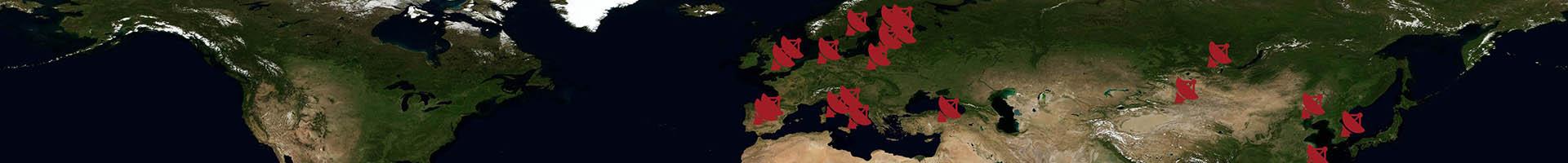
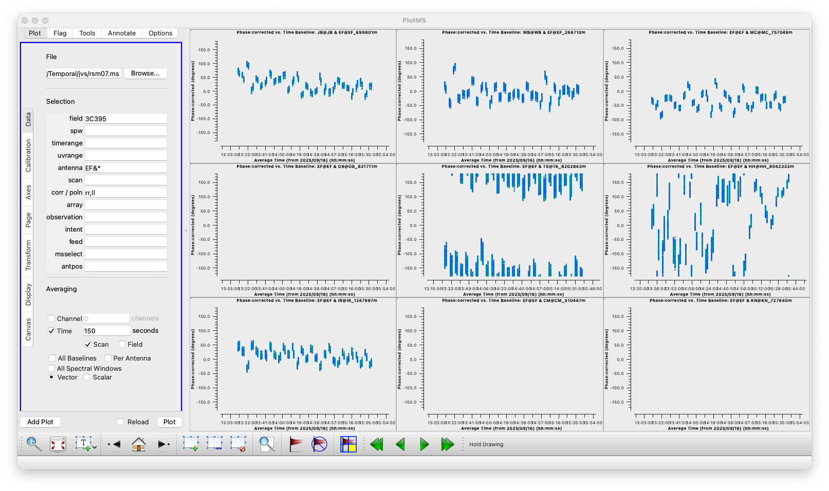
Let's make use of plotms to plot our data in different ways so we can get extra information on how it looks. Note that we recommend first to look at the plots that are in the EVN Archive, under 'standard plots' to safe same time. In particular,
- the "cross-" plots show the amplitudes vs frequency for a particular scan on the fringe-finder for all baselines to Effelsberg. You can see how the signal in the RR and LL polarizations is much stronger while the cross-polarizations (RL, LR) is near zero. The only reason why it is not zero is because of leakage existing at the different antennas (as they are not ideal instruments). Additionally, you can see how DE only contains data in two of the four subbands (as mentioned in the PI letter), and O8 does not show signal, as it was sending data but the antenna was stowed due to strong winds (and thus not pointing to the source). From here you can see how the signal at the edge of the subbands drops to nearly zero. Which we will flag just below.
- The ampphase- plots show the amplitudes and phases along time for the baselines to Effelsberg. This plot shows us what we knew about e.g. CM not getting actual data, DE stopping around the middle of the observation.And you can see how the fringe finder (blue color) is a much stronger source than the phase calibrator/target source.
flagdata(msfile, mode='manual', spw='*:0~3;60~63')
With this we remove the channels that are at the edge of each subbands, as the sensitivity there quickly drops to zero.
default(plotms)
vis=msfile
xaxis='time'
yaxis='amp'
field=phasecal
antenna='EF&*'
corr='rr,ll'
gridrows=3
gridcols=3
iteraxis='baseline'
coloraxis='corr'
plotms()
We can see in the plots below how all the data seems to be quite smooth (consistent amplitudes along the observation, and depending on the baseline more or less scatter due to the different sensitivities of the baselines), except some spikes at some particular times. The two colors (gray and blue) show the two polarizations (RR and LL) and both are also consistent with each other. You can follow the explanations at the DARA tutorial on EVN data on the different plots that you can create and how to identify the bad data that should be removed (you would expect the same data along the whole observations and thus any difference from the average profile means that either there was radio frequency interferencies (RFI, resulting in spikes at some times/frequencies) or failures at the antenna level (if amplitudes drop significantly). Apart of those spikes, we do not spot anything else relevant at this stage.
By selecting an area with the button ![]() and retrieving the information about the selected visibilities with
and retrieving the information about the selected visibilities with ![]() , we can see how this particular spike is produced in JB&EF, only on the spw=0, and channels 54~59. We can thus flag only the data with this selection with flagdata. And similar procedure with the rest of the big spikes.
, we can see how this particular spike is produced in JB&EF, only on the spw=0, and channels 54~59. We can thus flag only the data with this selection with flagdata. And similar procedure with the rest of the big spikes.
Step 2: A Priori Amplitude Calibration
The first step in our calibration will be to calibrate the gains of the telescopes. For, that we will be using the a-priori system temperatures and gain curves from each telescope. This information is included in the MS file, and can actually be plotted in plotms by selecting 'Tsys' in the y axis. You will see that for this experiment, all telescope have constant values along the observations as we have prepared this information before the whole observing run was done and thus operators at the antennas could produce these files. But these are accurate enough to do a proper analysis.
We start by creating the calibration table that corrects for the system temperature values (which will scale the amplitudes of the visibilities to match physical units, i.e. Jansky units):
default(gencal)
vis=msfile
caltable='rsm07.tsys'
caltype='tsys'
uniform=False
gencal()
And the second part of this step is to correct for the gain curves (response of the telescopes at different elevations):
default(gencal)
vis=msfile
caltable= "rsm07.gcal"
caltype="gc"
gencal()
WARNING: if you have problems with the previous file (as during the school, although we have already fixed the original FITS-IDI files), instead of creating the gain curve table you can (download it from here and uncompress). There was a small bug in the GC information that we appended in this observation.
These two steps will create two calibration tables (rsm07.tsys and rsm07.gcal) that later will be applied to the data. Instead of applying them directly, we will be using all these tables on-the-fly for each future calibration step. This improves the speed of the data reduction (as applying these tables is expensive in CASA).
We can inspect Tsys corrections:
default(plotms)
vis='rsm07.tsys'
xaxis='frequency'
yaxis='tsys'
gridrows=3
gridcols=3
coloraxis='corr'
iteraxis='antenna'
plotms()
xaxis='time'
plotms()
As mentioned before, we are analyzing the project before the observing run actually finished, you will see that all Tsys values are the same along time, but different for each telescope. This is because the information is only generated after the run finishes. The Tsys values there are proportional to the sensitivity of each antenna.
flagdata()
flagdata(msfile, mode='quack', antenna='WB', quackinterval=2, quackmode='beg')
Step 3: Main Calibration
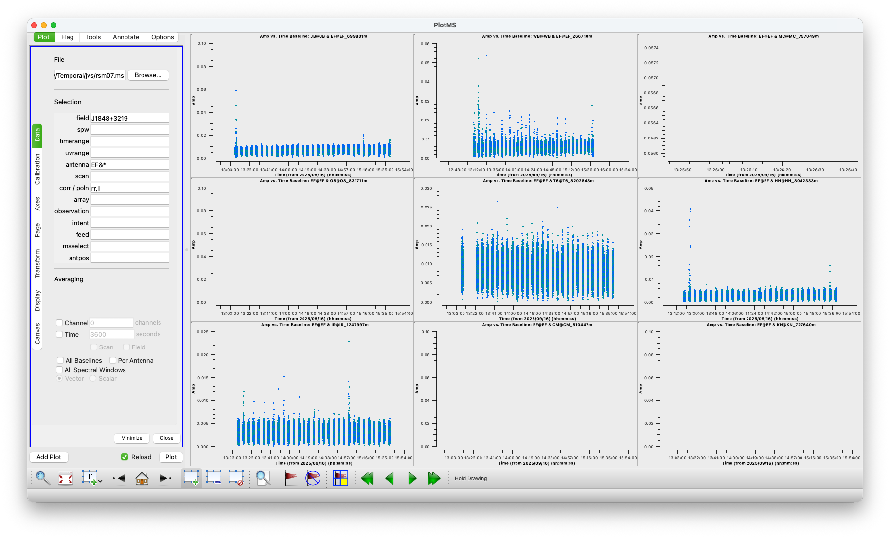
The first part of the calibration will involve correcting for the phases. First, we will correct for the instrumental delays: the jumps in phase that you see between subbands for some antennas. You should search for a good few-minutes of good data (without spikes, good signal, and more important all antennas) with plotms. Given that the fringe-finder is our strongest source, we can plot the amplitudes vs frequency for each of the scans on the fringe finder (that we know from the listobs() command. For example:
default(plotms)
vis=msfile
field=fringefinder
xaxis='frequency'
yaxis='phase'
ydatacolumn='data'
antenna='EF&*'
coloraxis='corr'
corr='rr,ll'
timerange='15:48:00~15:50:00'
averagedata=True
avgtime='120'
iteraxis='antenna'
gridrows=3
gridcols=3
plotms()
As this is a short observations and all antennas were observing in all scans, picking one of another time is not too relevant. But in other real observations, you may have some of the scans on the fringe finder where some antennas did actually not observe. In such case, this will determine with scan to pick. You want to select a few minutes of data including all antennas that observed. From standard calibrator sources, this already gives enough signal-to-noise, and you do not want longer times as then there may be time variability in the phases.
We run fringefit to correct for these instrumental delays (SBD: Single Band Delays):
default(fringefit)
vis=msfile
caltable='rsm07.sbd'
timerange='15:48:00~15:50:00'
solint='inf'
zerorates=True
refant='EF'
minsnr=10
gaintable=['rsm07.gcal','rsm07.tsys']
interp=['nearest','nearest,nearest']
parang=True
fringefit()
Note that here we are selecting 2 min of data via timerange, and deriving only one solution for such interval (solint='inf'), as we are doing this under the condition that there is no time variability. Furthermore, the zerorates=True tells fringefit not to correct for the rates (evolution of the phases along time). With this we ensure that we will be only correcting for the delays. The gaintable and interp tells fringefit to take into account the previous calibration steps that we have already performed.
At the end of the execution, in the message log you will see:
2025-09-29 13:28:54 INFO fringefit	Calibration solve statistics per spw:  (expected/attempted/succeeded):
INFO fringefit	  Spw 0: 1/1/1
INFO fringefit	  Spw 1: 1/1/1
INFO fringefit	  Spw 2: 1/1/1
INFO fringefit	  Spw 3: 1/1/1
Implying that it got one succesful solution per SPW, as expected. You will also see some warning messages in red indicating that some spw for some antennas did not contain solutions are were flagged (antenna 6 and 10, all four spws). But those are the antennas that could not participate in the observation and did not have data, as we saw at the beginning.
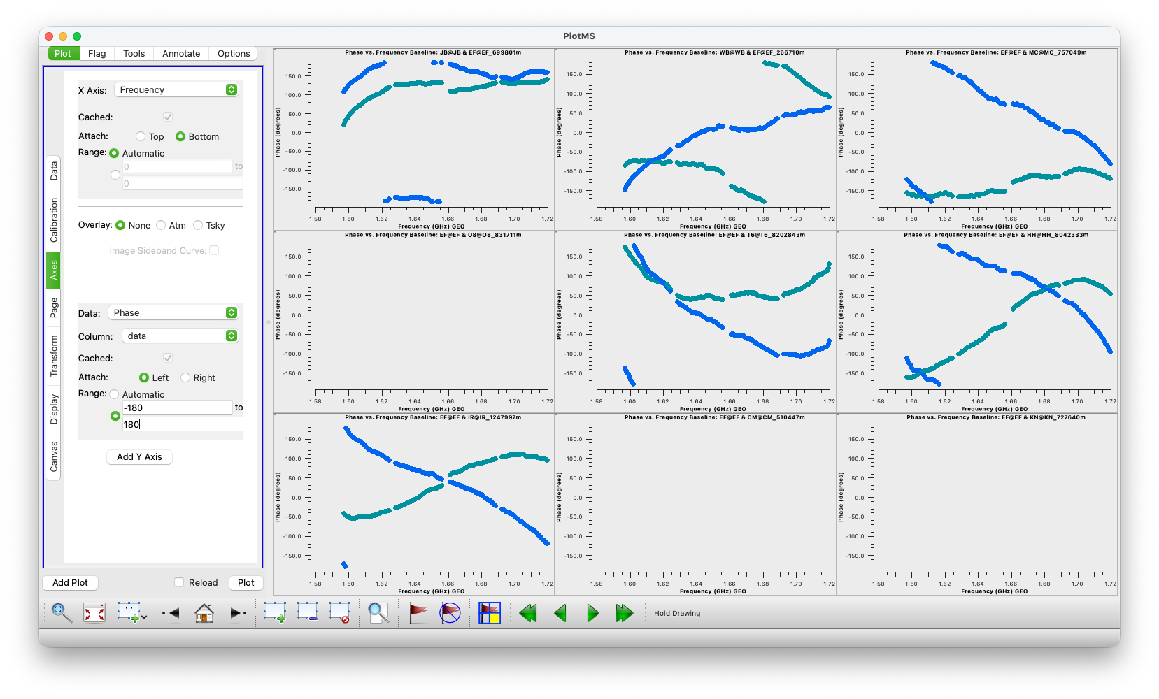
We will now apply the SBD solutions to our data. We will be using all tables we have created up to now and apply to the full dataset:
default(applycal)
vis=msfile
gaintable=['rsm07.gcal','rsm07.tsys','rsm07.sbd']
interp=['nearest','nearest,nearest','nearest']
parang=True
applycal()
And we can check how the solutions look like:
tget(plotms)
vis=msfile
timerange='15:48:00~15:50:00'
field=fringefinder
xaxis='freq'
yaxis='phase'
ydatacolumn='corrected'
antenna-'EF&*'
corr='rr,ll'
coloraxis='corr'
iteraxis='baseline'
gridrows=3
gridcols=3
scalar=False
avgtime=120
plotms()
Phases should not look around zero for the time when we corrected via the SBD. In the figures below we have set the y axis range from -180 to 180 degrees, and compared the DATA column (before calibration) and the CORRECTED column (after calibration). Try to plot another time range, and you will see how phases are no longer at zero (because we have not correct for the time evolution (zerorates=True), but the phases are always continuous from one subband to another.
Multi-band delays and rates (MBD):
Once we have corrected for the intrumental delays (phase jumps) between subbands for the different antennas, we will be able to correct for the evolution of the phases for the whole observation. As we saw from the previous plots, now the phases are continuous and thus we can combine all spw so the signal-to-noise (SNR) achieved for each solution will be higher than if we do not combine spw. In this case it is not critical as the sources are really bright, but in those cases where your phase calibrator is weak, this will produce better solutions.
For the multi-band correction, we will be computing the delay and rate solutions for all our calibrators (fringe finder and phase calibrator). This will allow us to 1) get both sources properly calibrated and 2) extrapolate the solutions from the phase calibrator to the target.
default(fringefit)
vis=msfile
caltable='rsm07.mbd'
field='J1848+3219,3C345'
solint='inf'
zerorates=False
refant='EF,MC'
combine='spw'
minsnr=7
gaintable=['rsm07.gcal','rsm07.tsys','rsm07.sbd']
interp=['nearest','nearest,nearest','nearest']
parang=True
fringefit()
While running, you will see the signal-to-noise (SNR) values obtained for each baseline (Ef to each antenna) for each scan and each polarization (aka correlation). In our case, the sources are extremely bright and thus the SNR values are between hundreds and tens of thousands. Note that each antenna has a different sensitivity and hence the broad range of different SNR values. At the very end, it will tell you that it found 33/33/33 (expected/attempted/succeeded) solutions, all of them in spw 0. For spw 1-3 you will see 0/0/0. This is because we are combining 'spw', and thus CASA only obtains one solution for the whole bandwidth, and stores it in the first spw.
You can first inspect the MBD solutions:
default(plotms)
vis='rsm07.mbd'
xaxis='time'
yaxis='delay'
gridrows=4
gridcols=4
coloraxis='corr'
iteraxis='antenna'
plotms()
And same for 'rates'. Solutions should be smooth in time and any outlier can be directly flagged in plotms.

Then, we can apply the solutions. In this case, we are correcting for (mostly) atmospheric affects and thus they depend on the pointing position. Hence, we can use the solutions on the fringe finder to correct itself, same for the phase calibrator, and then the target will be corrected from the solutions obtained on the phase calibrator.
default(applycal)
vis='rsm07.ms'
field='J1848+3219,3C345,3C395'
gainfield=['', '', '3C345', '3C345,J1848+3219']
gaintable=['rsm07.gcal','rsm07.tsys','rsm07.sbd','rsm07.mbd']
interp=['nearest', 'nearest,nearest','nearest','linear']
spwmap=[[],[],[],[0,0,0,0]]
parang=True
applycal()
And finally we correct for the bandpass (the response of each antenna within each subband). While this is in theory a purely amplitude-related correction, it is recommended to do it after fringe fit because internally it is correcting for the complex numbers. Because of that, if the phases are not corrected, it may have an effect into the solutions.
default(bandpass)
vis=msfile
caltable='rsm07.bpass'
field=fringefinder
gaintable=['rsm07.gcal','rsm07.tsys','rsm07.sbd','rsm07.mbd']
interp=['nearest','nearest,nearest','nearest','linear']
solnorm=True
solint='inf'
refant='EF'
bandtype='B'
spwmap=[[],[],[],[0,0,0,0]]
parang=True
bandpass()
We apply the solution to all calibrations:
default(applycal)
vis=msfile
field=''
gaintable=['rsm07.gcal','rsm07.tsys','rsm07.sbd','rsm07.mbd','rsm07.bpass']
interp=['nearest','nearest,nearest','nearest','linear','nearest,nearest']
spwmap=[[],[],[],[0,0,0,0],[]]
parang=True
applycal()
And we inspect the corrected data:
default(plotms)
vis=msfile
xaxis='frequency'
yaxis='amp'
coloraxis='corr'
iteraxis='antenna'
plotms()
Only a few outliers are seen (e.g. see the selected area in the plot below), which can be flagged directly in the plot. Otherwise all amplitudes and phases seem quite stable. A slow amplitude increase is seen in a few baselines, which it may be produced due to the increasing elevation of the source above the horizon with time. This could be corrected for during the self-calibration.
Step 4: Export Data
At this stage it is recommended to produce a MS with the whole calibration applied. In this sense, we will not need to apply all tables again and we will be able to return easily to this stage if needed. To do that we will split the data, creating a single MS for each source and taking the 'corrected' data. We will also average all channels per subband to reduce the data (note that this will actually reduce our effective field of view, but still big enough for our target sources):
# Phase calibrator
default(mstransform)
vis=msfile
outputvis='rsm07_J1848+3219.ms'
field='J1848+3219'
datacolumn='corrected'
keepflags=True
chanaverage=True
chanbin=64
mstransform()

# Target
default(mstransform)
vis=msfile
outputvis='rsm07_3C395.ms'
field='3C395'
datacolumn='corrected'
keepflags=True
chanaverage=True
chanbin=64
mstransform()
We will not be spliting the fringe finder here as it is not longer relevant for our science. But in case you want to get an image from that source, you can also export it and later image it.
Step 7: Imaging the data
For more details on this process, look at the slides on imaging and self-calibration.
tclean(vis='***',
       imagename='***',
       specmode='mfs',
       niter=1500,
       cycleniter=300,
       threshold=0,
       imsize=['**','**'],
       cell='**',
       weighting='**',
       deconvolver='**',
       savemodel='modelcolumn',
       interactive=True)
In MacOS:
from casagui.apps import run_iclean
run_iclean(vis=target+'.ms',
	   imagename='***',
	   specmode='mfs',
	   niter=1500,
	   cycleniter=300,
	   threshold=0,
	   imsize=['**','**'],
	   cell='**',
	   weighting='**',
	   deconvolver='**',
	   savemodel='modelcolumn')
ft(vis=target+'.ms',
   model='***.model',
   usescratch=True)
Step 6: Self Calibration
After imaging, the MS will now contain the model that you computed for your source.
You can look at the model in plots:
plotms(vis=target+'.ms', xaxis='uvdist', yaxis='amp', ydatacolumn='model', correlation='RR,LL', avgchannel='16', coloraxis='spw', plotfile='', overwrite=True)
Then you can derive the calibration table. First start with a long solution interval and to correct only for the phases.
gaincal(vis=target+'.ms', calmode='p',caltable='target-sc-p1', field=target, solint='10min',refant='EF', minblperant=3, minsnr=5)
The calibration table should contain corrections that are on a small level, and you can check with:
plotms(vis='target-sc-p1', gridcols=2, gridrows=3, xaxis='time', yaxis='phase', iteraxis='antenna', coloraxis='spw', plotrange=[-1,-1,-180,180])
Apply the calibration:
applycal(vis=target+'.ms', gaintable=['target-sc-p1'])
Then you can repeat the cycle of imaging (it should look slightly better now), and self calibration in phase with a shorted interval (2min, as you do not expect faster changes due to the atmosphere).
After another imaging round, if the solutions (in plots) seem to converge to just small improvements, one can run the self-calibration in amplitude and phase. In this case, running gaincal with calmode='ap' . For amplitude, you do not expect fast changes, but only on the order of ~30 min or more. Therefore a longer solution interval of half an hour or one hour is enough.
The final image with this corrections should look much better!