EVN Data Reduction Guide

Become familiar with EVN data reduction in AIPS or CASA. Here you can find the basic commands to calibrate your EVN data using any of the two packages (AIPS instructions on the left column, CASA instructions on the right column). Hover your mouse over the different parameters to know their meaning and the explanation about the chosen values. Note that VLBI data reduction under CASA is still under heavy development, and thus several options available in AIPS may still be missing in CASA.
You can also access the EVN Data Reduction Tutorials to follow a hands on calibration.

First steps.
Inspecting the data.
Calibration:
Split the data.
Imaging.
Post-imaging steps:
- Image fitting and statistics.
- Self-calibration.
Specific observing modes:
- Multi phase-center observations.
- Primary beam corrections.
Frequently Asked Questions (FAQ).

Obtaining the data

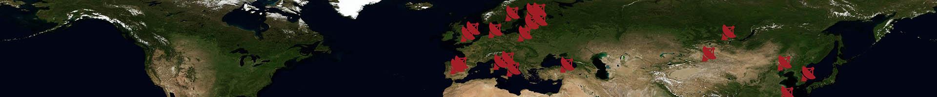
The very first step is to obtain your EVN data, that can be retrieved from the EVN Data Archive. See the detailed instructions from the EVN Data Access page.

The EVN Data Archive allows you to access the FITS-IDI files with the correlated data, the EVN Pipeline results (not scientific ready results!), and the feedback and check plots from the observation. The EVN Data Archive webpage is divided in the following sections:

Feedback page, containing the feedback coming directly from each station and provides information about local circumstances during the observation.
Logfiles page, containing the station logfiles, schedule files, and all detailed instrumental settings during the observation.
Standard plots, showing the quality of the correlated experiment. These plots are produced after the correlation and show the behavior of the stations along the observation. We recommend to take a look at these plots to get a good feeling on how all stations performed. Additionally, under the letter to the P.I. link, you will find a useful feedback from the EVN support scientist that processed your observation. This is the same information that you would have received by email if you are the PI.
Pipeline results, providing a more detailed impression of the quality of the data. It contains plots for each source separately. Whereas the final results from the pipeline should not be considered for scientific results, we encourage the users to use the a-priori amplitude calibration table (CL2) and flag table (FG1) from the pipeline to start a manual calibration (see below).
FITS files with the correlated data in FITS-IDI format.

All these results would provide a good feedback about the data during the observation. To start the data reduction you will need to download the FITS-IDI files with all the data, and then the following files (depending on with which software you are performing the data reduction):

With AIPS: download the AIPS calibration tables from the EVN Pipeline (experiment_name.tasav.FITS file; click in the Pipeline tab and then right click in AIPS calibration tables). This file contains the calibration tables that have been applied to your data in the Pipeline, and you can find a more detailed summary of which may be found in the Short summary of CL/SN table contents section. We recommend to apply the CL2, FG1 (a-priori calibration and flagging tables), and in general BP1 (bandpass calibration). This will help you with a smoother start of the calibration, while the following steps are better to be done manually.
With CASA: If you are analyzing observations after January 2022, then you will only need to download the a-priori flagging table (UVFLG flagged data file under the Pipeline tab). The a-priori gain calibration will already be contained within the FITS-IDI files. However, if you are calibration an older observation, then you will also need to download the Associated EVN calibration file (also under the Pipeline tab).

Start AIPS and load the data

AIPS can be started by typing (you may need to initialize the environment before hand): aips tv=local:0. Introduce the AIPS user number that you wish to use for the session.

The EVN data need to be loaded as:

default fitld
datain 'PWD:experiment_1_1.IDI
digicor -1
doconcat 1
ncount n
outname 'exp'
go fitld
recat

Fix the list of scans:

default extdest
getn 1
inext 'NX'
go extdest

task 'indxr'
go indxr

And the same for the tasav FITS file:

tget fitld
datain 'PWD:experiment_tasav.FITS
digicor -1
doconcat -1
ncount 1
outname 'exp'
go fitld

The useful calibration tables from the EVN Pipeline must be transfered from the tasav file to the data. In the case of EVN data, this means the CL table no. 2 (calibration table containing the parallactic angle and a-priori gain corrections), the a-priori flagging (FG) table, and, optionally, the bandpass (BP) calibration.

default tacop
getn 2
geton 1
inext 'CL'
invers 2
ncount 1
go tacop

tget tacop
inext 'FG'
invers 1
ncount 1
go tacop

Optionally the bandpass calibration from the EVN Pipeline can be copied. Otherwise a manual bandpass calibration may be preferred.

tget tacop
inext 'BP'
invers 1
ncount 1
go tacop

Start CASA and load the data

Before starting CASA it is required to download the external CASA VLBI Python module located under this link, which will append calibration meta-data (system temperature, gain, flags) to the FITS-IDI file.

Note that appending system temperature and gain curve information is only required if you are analyzing observations older than 1 January 2022. Otherwise this information is already available in the provided FITS-IDI files. Running the module scripts will notify you of this and not alter any existing data. You will still need the module to convert the UVFLG information.

To import the module in CASA, set your $PYTHONPATH variable to point to the directory where you have saved the downloaded module.

You need another two files from the EVN Data Archive in addition to the previously mentioned FITS-IDI files. Under the "Pipeline" tab, download both the Associated EVN calibration (ANTAB file) and the UVFLG flagged data (uvflg file).

Now CASA can be started by typing casa. For proper functionality of the CASA VLBI module, make sure you run the most recent CASA distribution with the highest Python version.

To import the module at the CASA prompt type

from casavlbitools import fitsidi

Generate a sorted list of all your FITS-IDI files

from natsort import natsort_keygen

import glob

myidifiles = sorted(glob.glob('experiment*IDI*'),key=natsort_keygen())

The natsort module may need to be separately installed, you need this to get natural sorting if you have more than 9 FITS-IDI files.

First the system temperature information is added. This requires a list of all the FITS-IDI files in the variable idifiles.

fitsidi.append_tsys('experiment.antab',myidifiles)

The module will give an error if there is already system temperature information present in the FITS-IDI files. This is normal behaviour. Depending on the size of your FITS-IDI files and your machine CPU/memory, this can take anywhere from a few minutes to ~half an hour. Be patient.

Second, this is repeated with the gain curve information.

fitsidi.append_gc('experiment.antab',myidifiles[0])

Note the subtle difference: appending the gain curve requires only one of the FITS-IDI files. As above, this module gives an error if the gain information is already present, which is also benign. This step is fast.

Finally, the UVFLG flags from the archive need to be converted into a CASA readable format. This module writes the flags to a file in your working directory.

fitsidi.convert_flags('experiment.uvflg', myidifiles, outfile=experiment.flag)

Now the IDI FITS files may be converted to a Measurement Set (MS) file, the native format for CASA:

importfitsidi(vis='experiment.ms',
    fitsidifile=myidifiles,
    constobsid=True,
    scanreindexgap_s=15.0)

The flag table may be applied to the data:

flagdata(vis='experiment.ms',
    mode='list',
    inpfile='experiment.flag',
    reason='any',
    action='apply',
    flagbackup=True,
    savepars=False)

And an a-priori gain calibration may be generated with:

gencal(vis='experiment.ms',
    caltable='cal.tsys',
    caltype='tsys',
    uniform=False)

gencal(vis='experiment.ms',
    caltable='cal.gcal',
    caltype='gc')

Note that CASA handles differently the parallactic angle corrections. They are applied on-the-fly for each calibration task instead of being corrected at the beginning like in AIPS.

Inspect the data

First, information about the number of scans, times, sources, and antennas can be retrieved by

In AIPS:

default listr
getn 1
optype 'SCAN'
go listr

default prtan
getn 1
go prtan

Data should be checked carefully before calibration to identify possible issues like radio frequency interference (RFI), dropouts of stations and some particular times, or bad data in general. We recommend to do a manual flagging of the data at this point and indentify the edge channels where the signal already dropped (and should thus be flaged). AIPS has a large number of possible tasks to perform these steps, among others UVPLT/UVFLG, SPFLG, or TVFLG. Pick your preferred one.

In CASA:

listobs(vis='experiment.ms')

And you can visualize the data interactively with

plotms(vis='experiment.ms')

Among other options, you can set the parameters xaxis, yaxis, coloraxis (either when calling plotms or inside the interactive window) to display different information like amplitudes, phases, times, uv distances, or u versus v. This tool also allows you to flag the bad data.

Atmospheric corrections

Depending on the data to be analyzed, some atmospheric corrections may be recommended. If the observation was conducted at frequencies of around 5 GHz or below, the data may suffer from ionospheric dispersive delays (different at each antenna and proportional to the Total Electron Content, TEC, along the line of sight and inversely proportional to the square of the frequency) that can be compensated.

In AIPS vlbatecr downloads the required ionospheric data at the time of the observation and produces a calibration.

run vlbautil
default vlbatecr
getn 1
go vlbatecr

A new CL table should have been created (number 3 if no additional steps have been done up to now).

In CASA tec_maps downloads the required data:

from casatasks.private import tec_maps
tec_image, tec_rms_image, plotname = tec_maps.create(vis='experiment.ms', doplot=True)

gencal(vis='experiment.ms', caltable='cal.tecim',
    caltype='tecim', infile='tec_image')

viewer('experiment.ms.IGS_TEC.im')
viewer('experiment.ms.IGS_RMS_TEC.im')

If the observation was conducted at frequencies above 20 GHz, you may want to correct for tropospheric effects.

Removing instrumental delay

Phase jumps between subbands (or IFs) are related to instrumental delays at each telescope and thus can be corrected by using the data from one of the strong calibrators and apply the solutions for the whole observation. Note that if the data only have one subband (or if you conduct a subband-independent global fringe calibration), this step is not necessary.

In AIPS:

default fring
getn 1
timerang d1 h1 m1 s1 d2 h2 m2 s2
docal 1
gainuse n
doband 1
bpver 1
weightit 1
refant a
solint 0
dparm(9) 1
snver 1
go fring

In CASA:

fringefit(vis="experiment.ms",
    caltable="cal.sbd",
    timerange='h1:m1:s1~h2:m2:s2',
    solint='inf',
    zerorates=True,
    refant='a'
    minsnr=10,
    gaintable=['cal.tsys', 'cal.gcal', ...]
    parang=True)

In AIPS look at the solutions with

default snplt
getn 1
inext 'SN'
invers 1
opty 'dela'
dotv 1
nplots 8
tvini
go snplt

In CASA look at the solutions with:

plotms(vis='cal.sbd',
    xaxis='frequency',
    yaxis='phase',
    antenna='a'
    correlation='rr,ll',
    timerange='h1:m1:s1~h2:m2:s2',
    averagedata=True,
    avgtime='120')

Note that they can also be plotted by using the plotcal function.

In AIPS apply the solutions to the data and create a new calibration (CL) table.

default clcal
getn 1
gainver n
gainuse n+1
snver 1
interpol ''
opcode 'cali'
refant a
go clcal

In CASA apply the calibration to the data.

applycal(vis='experiment.ms',
    gaintable=['cal.tsys', 'cal.gcal', 'cal.sbd', ...],
    parang=True)

NOTE: In some cases it is not possible to obtain a time range at which all stations were observing. In those cases multiple FRING instances must be run. In AIPS, run the first FRING exactly in the same way but use optype 'CALP' when running CLCAL with above settings (so it keeps data from antennas with no solutions in the previous SN table, i.e. the stations that did not observe in the considered scan).
Then run FRING again for a different time range where the remaining station(s) observed. In this case you need to run the task with the following parameters:
default fring
getn 1
timerang d1 h1 m1 s1 d2 h2 m2 s2
docal 1
gainuse n
doband 1
bpver 1
weightit 1
refant a1
dofit a2, a3,...
antenna a1, a2, a3,...
solint 0
dparm(9) 1
snver s
go fring
default clcal
getn 1
gainver n
gainuse n+1
snver s
interpol ''
opcode 'calp'
refant a1
antenna a2, a3,...
go clcal
Repeat these steps (FRING and CLCAL) as many times as required to get solutions for all antennas.

Bandpass calibration

In AIPS the bandpass table can be imported (highly recommended) from the EVN Pipeline results with TACOP (previous steps). In some cases, a manual bandpass calibration must be performed to recover a flat response of the instruments across all the band:

default bpass
getn 1
calsour 'bandpass-calibrator',''
docal 1
gainuse n
refant a
solint -1
weightit 1
soltype 'l1r'
bpassprm(1) 0
bpassprm(2) 1
bpassprm(10) 1
go bpass

NOTE: You should pick the same scan used for the instrumental delay calibration. Otherwise, the bandpass calibration should be done after the global fringe-fitting (following step). In any case, note that the bandpass correction may introduce again some offsets between subbands/IFs. Therefore, it is recommended to run again the instrumental delay correction (and/or global fringe-fit) afterwards.

In CASA the manual bandpass calibration must be performed by running:

bandpass(vis='experiment.ms',
    caltable='cal.bpass'
    field='bandpass-calibrator',
    gaintable=['cal.tsys', 'cal.gcal', ...],
    solnorm=True,
    solint='inf',
    refant='a',
    bandtype='B',
    parang=True)

Global fringe (or frequency and time-dependent phase calibration)

Phases must be corrected for the whole observation. For VLBI data that means that delays and rates must be corrected by using fringe fit. If the target source is bright and compact enough, it can directly be used in the fringe-fit. However, in most of the cases a nearby calibrator (the so-called phase calibrator) should be used for that and then solutions must be extrapolated to the target source position.

In AIPS:

default fring
getn 1
calsour 'calsource1', 'calsource2', ''
docal 1
gainuse n
doband 1
bpver 1
timerang 0
weightit 1
refant a
solint t
aparm(5) 1
aparm(6) 3
aparm(9) 1
dparm 1 200 50 0
search a2, a3, a4
snver 2
go fring

In CASA:

fringefit(vis='experiment.ms',
    caltable='cal.mbd',
    solint='t',
    combine='spw',
    field='calsource1, calsource2,...',
    refant='a',
    minsnr=7,
    gaintable=['cal.tsys', 'cal.gcal', 'cal.bpass', 'cal.sbd', ...],
    parang=True)

Note that the solution interval (solint) should be long enough to produce solutions with a good signal-to-noise ratio, but it must be smaller than the time interval at which you see a significant phase evolution (which would de-correlate the signal). Typically it is of the order of a few minutes for standard arrays and EVN frequencies. Also note that it is not possible to combine IFs (aparm(5) 1 in AIPS or combine='spw' in CASA) if the instrumental delay correction was not performed beforehand.

In AIPS apply the solutions to the data and create a new calibration (CL) table. It is recommended to apply the solutions to one source at the time:

default clcal
getn 1
calsour 'sourceN' ''
source calsour
gainver n
gainuse n+1
snver 2
interpol 'self'
opcode 'cali'
refant a
go clcal

Repeate to all sources used in fring. Then if solutions must be transfer to the target (like in phase-referencing experiments) then:

tget clcal
calsour 'phaseCalibrator' ''
source 'target'
interpol 'ambg'
opcode 'cali'
refant a
go clcal

In CASA apply the calibration to the data:

applycal(vis='experiment.ms',
    gaintable=['cal.tsys', 'cal.gcal', 'cal.bpass', 'cal.sbd', 'cal.mbd', ...],
    spwmap=[[], [], [], N*[0], ...],
    parang=True)

NOTE: Fringe fit assumes that your source(s) are point-like (unresolved for all baselines) and located at the phase center position. However, in some cases this may not be true and a source model can be provided to for a more accurate fit. In FRING (in AIPS), add the parameters get2n i (where i refers to the image file of the source) and cmethod 'dft' (for a better model interpolation).

In the case of spectral line observations, CVEL may be executed to provide the conversion between frequencies and velocities.

Split and store the data

The final calibration may be applied to the data and different datasets can be produced for the different sources.

In AIPS:

default split
getn 1
source ''
docal 1
gainuse n
doband 1
bpver 1
flagv 0
aparm 2 0
go split

To store the UVDATA outside AIPS:

default fittp
getn i
dataout 'PWD:filename.uvfits'
go fittp

In CASA:

split(vis='experiment.ms',
    field='source_name',
    outputvis='source_name.ms',
    datacolumn='corrected')

To store the data as UVFITS:

exportuvfits(vis='filename.ms',
    field='sources',
    fitsfile='filename.uvfits',
    datacolumn='corrected')

Initial imaging

Now images for each source can be produced. Depending on the type of observations, the required parameters may differ significantly. In the case of continuum data, an image can be obtained with:

In AIPS:

default imagr
getn n
imsize 512
cellsize c
niter 10000
gain 0.05
cmethod 'dft'
robust r
dotv 1
go imagr

In the case of spectral line data, a cube may be wanted. Select multiple channels with the desired averaging to obtain it.

In CASA:

tclean(vis='filename.ms',
    field='source',
    imagename='source.image',
    specmode='mfs',
    nterms=1,
    deconvolver='hogbom',
    gridder='standard',
    imsize=1024,
    cell='XXmas',
    weighting='natural',
    niter=10000,
    interactive=True,
    savemodel='modelcolumn')

Image fitting and statistics

Different measurements can be performed in the obtained images. The most basic ones are:

In AIPS:

tvall: show the image.
imstat: provides the statistics of the image (like rms, maximum and minumum brightnesses).
tvstat: similar to imstat but a region in the image can be specified.
jmfit: fit a Gaussian to the image.

To store the FITS images outside AIPS:

default fittp
getn i
dataout 'PWD:filename.fits'
go fittp

In CASA:

imview or viewer: show the image and allows interactive measurements.
imstat: provides the statistics of the image (like rms, maximum and minumum brightnesses).
imfit: fit a Gaussian to the image.

To store the images as FITS files:

exportfits(imagename='imagefilename',
    fitsname='imagefilename.fits')

Self-calibration

Typically this calibration can still be improved by self-calibrating the target data (or the phase calibrator data and then transfer the solutions to the target if this is faint). If a good source model has already been created, then this one can be used to improve the calibration:

In AIPS:

default calib
getn n
get2n m
nmaps 1
refant a
weightit 1
soltype 'l1r'
cmethod 'dft'
solint t
aparm 3 0
solmode 'p'
go calib

It will create a CALIB file with the calibrated data which can be used to image again the source (now with a better calibration). Repeat this process iteractively until reaching the best possible calibration. After some rounds of phase-only selfcalibration, and only if the model is good enough, a phase-and-amplitude selfcalibration may be performed (setting solmode 'a&p').

If the selfcalibration has been performed in a calibrator source, then the solutions may be transfered to the original UVDATA file and applied to the target source, to be later on imaged again.
First the SN table created in the SPLIT file used for the selfcalibration must be copied to the original UVDATA:

default tacop
getn n
geton 1
inext 'SN'
invers s
ncount 1
outvers 0
go tacop

Now a new CL (calibration) table may be created with CLCAL in the same way as before by using this SN table. Split the target source data again applying this CL table and the fully calibrated dataset will be ready to be imaged.

In CASA: (NOTE: THIS SECTION IS UNDER TESTING)

gaincal(vis='filename.ms',
    caltable='cal.pcal'
    field='calibrator',
    gaintype='T',
    solint='inf',
    refant='a',
    calmode='p',
    combine='spw',
    minsnr=10,
    minblperant=4)

Apply the calibration:

applycal(vis='filename.ms',
    caltable='cal.pcal'
    field='sources',
    gainfield='calibrator',
    gaintable=['cal.pcal'],
    calwt=False,
    flagbackup=False,
    interp='linearperobs')

Repeat this process iteractively until reaching the best possible calibration. After some rounds of phase-only selfcalibration, and only if the model is good enough, a phase-and-amplitude selfcalibration may be performed (setting calmode='ap').

Multi phase-center observations

The EVN supports multi phase-center correlations, where different correlations at different positions (within the primary beam) can be performed to observe multiple source with only one pointing. In these cases, the calibration may be performed in the same way for only one phase center. Once it is done, you can apply the same calibration to the other phase centers.

Primary beam corrections

When you image a source that is significantly offset from the phase center (the position in the sky where all antennas were pointing to; like in the case of multi phase-cetner observations), you may need to correct your data for the primary beam of each individual antenna (their response pattern outside the pointing position). For observations correlated after January 2021, JIVE directly provides these corrections within the calibration tables produced by the EVN Pipeline. You only need to copy the SN #2 (table containing the amplitude corrections to apply for each antenna and source) and apply them to your data during the data reduction.

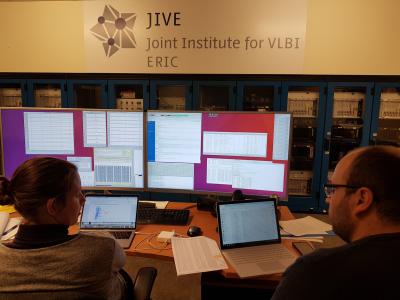
For older observations, please contact the EVN Support Scientists at JIVE (usersupport (at) jive.eu) to get information about how to apply this correction in your case.

Frequency Asked Questions (FAQ)

Uncertainties in total flux densities in VLBI data

Amplitudes in VLBI data are based on the measurement of antenna sensitivities and system temperatures during the observation. Given that no reference source can be used to set the true amplitude level (like it is done in connected interferometers with the known amplitude calibrators), the final amplitudes fully rely on these measurements and estimations. There is thus an uncertainty that propagates to the final absolute flux density scale in your data. Although it cannot be easily measured, in VLBI observations this method is typically accurate up to 10-15%. This should thus be the uncertainty quoted in the absolute flux density measurements that you perform on your data.

How to measure flux densities from the data

There are typically two different approaches to measure the flux density of a source in your VLBI data: doing it in the image plane or in the uv plane.

WARNING on change the phase center position in EVN Data with CLCOR

The use of CLCOR in AIPS to move the phase center of your data to a different position may produce incorrect shifts in the uv data if it is not performed cautiously. The issue raises due to the way that the reference epochs and positions internally (EOPOS and APPPOS tables). EVN data already contains a more accurate apparent position of the sources for the given epoch, but AIPS tries to recompute this one internally, creating an offset that is relevant when using CLCOR. To avoid this behavior, one needs to let AIPS to update the source position in the SU table to the correct one which is included in the EVN data. For that, the best way is to force a small dummy shift in the coordinates and undo it. After that, you can safely run CLCOR to compute the shift you need.
This dummy shift can be achieved with the following recipe:

default clcor
getn 1
sources 'A_SOURCE'
opcode 'ANTC'
clcorprm(6) = 0.1   # only a small shift of 0.1 arcsec
gainver 2    # assuming 2 is the highest available CL table
gainuse 3
go clcor

#Delete Cl table
default extdest
getn 1
inext 'CL'
invers 3
extdest

# To update SU table to the correlated position, and undoing the shift
default clcor
getn 1
sources 'A_SOURCE'
opcode 'ANTC'
clcorprm(6) = -0.1
gainver 2
gainuse 3
go clcor

#Delete CL table
go extdest

Gain calibration issues

In some data it may happen that one (or some) antennas exhibit a significant offset in the gain calibration, producing amplitudes that are significantly off from what it was expected (e.g. when compared to the other baselines). This issue can be corrected via self-calibration (producing an accurate model with the other baselines), or with tasks like gscale in packages like Difmap.

When do self-calibration?

Self-calibration can only be reliably used when certain conditions are met. You can read the guide from Sabrian Stierwalt (NRAO) about when, why, and how to do self-calibration on your data.